Real cycling data walkthrough¶

This notebook processes genuine battery-cycling data: the small vendored test fixture tests/data/cycler_cc_harmonized_raw.parquet (10 261 rows, 18 cycles of constant-current cycling, originally recorded at IFE, Norway). It uses the CellpyCellCore class, which orchestrates the engine and adds C-rates and half-cell cycle modes on top of the plain quickstart pipeline.

Run it from a checkout of the repository so the fixture path resolves.

from pathlib import Path

import matplotlib.pyplot as plt
import polars as pl

from cellpycore import CellpyCellCore, Data

FIXTURE = Path("../../tests/data/cycler_cc_harmonized_raw.parquet").resolve()
raw = pl.read_parquet(FIXTURE)
print(f"{raw.height} rows, {raw.width} columns")

10261 rows, 29 columns

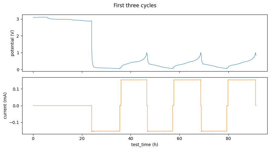
1. A first look at the raw data¶

The frame is already in the harmonized raw schema: potential in volts, current in amperes, times in seconds, capacities cumulative per cycle and direction.

raw.select(
    "datapoint_num",
    "test_time",
    "cycle_num",
    "step_num",
    "current",
    "potential",
    "cumulative_charge_capacity",
).head()

shape: (5, 7)

datapoint_num	test_time	cycle_num	step_num	current	potential	cumulative_charge_capacity
i64	f64	i64	i64	f64	f64	f64
1	300.010482	1	1	0.0	3.097617	0.0
2	600.014947	1	1	0.0	3.10008	0.0
3	900.026371	1	1	0.0	3.101312	0.0
4	1200.039773	1	1	0.0	3.102852	0.0
5	1500.051275	1	1	0.0	3.10316	0.0

first_cycles = raw.filter(pl.col("cycle_num") <= 3)
fig, (ax1, ax2) = plt.subplots(2, 1, figsize=(9, 5), sharex=True)
ax1.plot(first_cycles["test_time"] / 3600, first_cycles["potential"], lw=0.8)
ax1.set_ylabel("potential (V)")
ax2.plot(
    first_cycles["test_time"] / 3600,
    first_cycles["current"] * 1000,
    lw=0.8,
    color="tab:orange",
)
ax2.set_ylabel("current (mA)")
ax2.set_xlabel("test_time (h)")
fig.suptitle("First three cycles")
fig.tight_layout()

png

2. Process with `CellpyCellCore`¶

The class handles the cycle_mode string for you. This cell is an anode half-cell, so coulombic efficiency is computed in the inverted direction (CE = 100 * charge / discharge). make_core_step_table also estimates a per-step C-rate from nom_cap (absolute, in the same unit as capacity — pass your cell's real value).

NOM_CAP = 0.001  # Ah — nominal capacity of this small test cell

core = CellpyCellCore()
core.data = Data.from_raw_frame(raw)
core.cycle_mode = "anode"

data = core.make_core_step_table(core.data, nom_cap=NOM_CAP)
data = core.make_core_summary(data, current_conversion_factor=1.0)

print(f"steps:   {data.steps.height} rows")
print(f"summary: {data.summary.height} cycles")

steps:   103 rows
summary: 18 cycles

3. The step table¶

One row per sequential step with per-step statistics, the classified step_type, and the estimated C-rate.

data.steps.select(
    "cycle_num",
    "step_num",
    "step_type",
    "c_rate",
    "current_mean",
    "potential_first",
    "potential_last",
).head(8)

shape: (8, 7)

cycle_num	step_num	step_type	c_rate	current_mean	potential_first	potential_last
i64	i64	str	f64	f64	f64	f64
1	1	"ocvrlx_down"	0.0	0.0	3.097617	2.88916
1	2	"ir"	0.00066	6.6289e-7	2.8907	2.8907
1	3	"discharge"	0.15221	-0.000152	2.839894	0.049894
1	4	"ir"	0.00004	-4.3646e-8	0.064366	0.064366
1	5	"ocvrlx_up"	0.0	0.0	0.0696	0.095465
1	6	"charge"	0.15362	0.000154	0.110245	1.000113
1	7	"ir"	0.00031	3.0962e-7	0.995803	0.995803
1	8	"ocvrlx_down"	0.0	0.0	0.990568	0.866787

data.steps.group_by("step_type").len().sort("len", descending=True)

shape: (5, 2)

step_type	len
str	u32
"ir"	33
"discharge"	18
"ocvrlx_down"	18
"ocvrlx_up"	17
"charge"	17

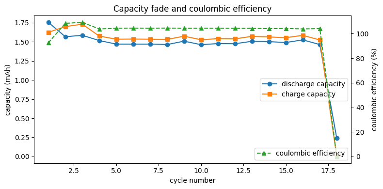
4. Capacity fade and coulombic efficiency¶

The per-cycle summary is where degradation trends live.

summary = data.summary
fig, ax1 = plt.subplots(figsize=(8, 4))
ax1.plot(
    summary["cycle_num"],
    summary["discharge_capacity"] * 1000,
    "o-",
    label="discharge capacity",
)
ax1.plot(
    summary["cycle_num"],
    summary["charge_capacity"] * 1000,
    "s-",
    label="charge capacity",
)
ax1.set_xlabel("cycle number")
ax1.set_ylabel("capacity (mAh)")
ax1.legend(loc="center right")

ax2 = ax1.twinx()
ax2.plot(
    summary["cycle_num"],
    summary["coulombic_efficiency"],
    "^--",
    color="tab:green",
    label="coulombic efficiency",
)
ax2.set_ylabel("coulombic efficiency (%)")
ax2.legend(loc="lower right")
ax1.set_title("Capacity fade and coulombic efficiency")
fig.tight_layout()

png

summary.select(
    "cycle_num",
    "charge_capacity",
    "discharge_capacity",
    "coulombic_efficiency",
    "charge_c_rate",
    "discharge_c_rate",
).head(6)

shape: (6, 6)

cycle_num	charge_capacity	discharge_capacity	coulombic_efficiency	charge_c_rate	discharge_c_rate
i64	f64	f64	f64	f64	f64
1	0.001625	0.001755	92.610791	0.15362	0.15221
2	0.0017	0.001567	108.426838	0.15361	0.15232
3	0.001732	0.001586	109.19373	0.15359	0.15232
4	0.001576	0.001517	103.86601	0.30553	0.30444
5	0.001535	0.001471	104.358191	0.30549	0.30439
6	0.001537	0.001471	104.517674	0.30547	0.30444

Next steps¶

core.add_scaled_summary_columns(...) adds gravimetric / areal / absolute variants of the capacity-like columns and a normalized (equivalent) cycle index — see the standalone-use guide.
make_core_summary(..., exclude_step_types=["cv_"]) builds a summary with the capacity contribution of matching step types subtracted.
The exact meaning of every output column is specified in the step table and cycle table documents.