Quickstart on mock data¶

This notebook runs the whole cellpy-core pipeline — Data.from_raw_frame → make_step_table → make_summary — on synthetic data, so it works anywhere the cellpycore package is installed (no cycler files needed).

The mock frame comes from cellpycore.testing.mock_data.create_raw_data, which produces 1000 rows of charge / discharge / rest steps in the harmonized raw schema.

import matplotlib.pyplot as plt

import cellpycore
from cellpycore import Data, make_step_table, make_summary
from cellpycore.testing.mock_data import create_raw_data

print(f"cellpycore version: {cellpycore.__version__}")

cellpycore version: 0.1.3

1. Create a raw frame¶

A raw frame is an ordinary polars DataFrame whose columns follow the harmonized raw schema (cellpycore.config.RawCols).

raw = create_raw_data()
raw.select(
    "test_time", "cycle_num", "step_num", "step_type", "current", "potential"
).head()

shape: (5, 6)

test_time	cycle_num	step_num	step_type	current	potential
f64	i64	i64	str	f64	f64
0.0	0	0	"charge"	1.0	3.7
1.0	0	0	"charge"	1.1	3.71
2.0	0	0	"charge"	1.2	3.72
3.0	0	0	"discharge"	-1.3	3.67
4.0	0	0	"discharge"	-1.4	3.66

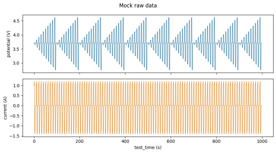
fig, (ax1, ax2) = plt.subplots(2, 1, figsize=(9, 5), sharex=True)
ax1.plot(raw["test_time"], raw["potential"], lw=0.8)
ax1.set_ylabel("potential (V)")
ax2.plot(raw["test_time"], raw["current"], lw=0.8, color="tab:orange")
ax2.set_ylabel("current (A)")
ax2.set_xlabel("test_time (s)")
fig.suptitle("Mock raw data")
fig.tight_layout()

png

2. Run the pipeline¶

Data.from_raw_frame is the validating front door: it checks that the frame carries the load-bearing columns with sane dtypes and reports every problem in a single error. Then the step table must be built before the summary, because make_summary reads data.steps.

data = Data.from_raw_frame(raw)
make_step_table(data, nom_cap=1.0)  # nom_cap (absolute, Ah) sets the per-step C-rate
make_summary(data)

print(f"steps:   {data.steps.height} rows")
print(f"summary: {data.summary.height} cycles")

steps:   100 rows
summary: 10 cycles

3. Inspect the step table¶

One row per sequential step, with per-step statistics (first / last / min / max / mean of current, potential, capacities …) and the classified step_type.

data.steps.select(
    "cycle_num",
    "step_num",
    "step_type",
    "current_mean",
    "potential_first",
    "potential_last",
    "charge_capacity_last",
    "discharge_capacity_last",
).head(8)

shape: (8, 8)

cycle_num	step_num	step_type	current_mean	potential_first	potential_last	charge_capacity_last	discharge_capacity_last
i64	i64	str	f64	f64	f64	f64	f64
0	0	"cv_discharge"	-0.04	3.7	3.709	0.33	0.37
0	1	"discharge"	-0.04	3.8	3.709	0.66	0.74
0	2	"discharge"	-0.04	3.9	3.709	0.99	1.11
0	3	"discharge"	-0.04	4.0	3.709	1.32	1.48
0	4	"discharge"	-0.04	4.1	3.709	1.65	1.85
0	5	"discharge"	-0.04	4.2	3.709	1.98	2.22
0	6	"discharge"	-0.04	4.3	3.709	2.31	2.59
0	7	"discharge"	-0.04	4.4	3.709	2.64	2.96

4. Inspect the per-cycle summary¶

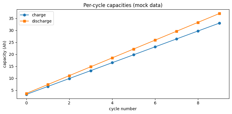
One row per cycle: capacities, coulombic efficiency, durations, and per-direction current / potential statistics.

data.summary.select(
    "cycle_num",
    "charge_capacity",
    "discharge_capacity",
    "coulombic_efficiency",
    "last_test_time",
)

shape: (10, 5)

cycle_num	charge_capacity	discharge_capacity	coulombic_efficiency	last_test_time
i64	f64	f64	f64	f64
0	3.3	3.7	112.121212	99.0
1	6.6	7.4	112.121212	199.0
2	9.9	11.1	112.121212	299.0
3	13.2	14.8	112.121212	399.0
4	16.5	18.5	112.121212	499.0
5	19.8	22.2	112.121212	599.0
6	23.1	25.9	112.121212	699.0
7	26.4	29.6	112.121212	799.0
8	29.7	33.3	112.121212	899.0
9	33.0	37.0	112.121212	999.0

summary = data.summary
fig, ax = plt.subplots(figsize=(8, 4))
ax.plot(summary["cycle_num"], summary["charge_capacity"], "o-", label="charge")
ax.plot(summary["cycle_num"], summary["discharge_capacity"], "s-", label="discharge")
ax.set_xlabel("cycle number")
ax.set_ylabel("capacity (Ah)")
ax.set_title("Per-cycle capacities (mock data)")
ax.legend()
fig.tight_layout()

png

Next steps¶

The real cycling data walkthrough runs the same pipeline on genuine instrument data via the CellpyCellCore class, adding C-rates and half-cell cycle modes.
The standalone-use guide documents the full contract the caller must honor.